2. Compute travel times
This notebook computes the travel times from all the points of a three-dimensional grid to each seismic station. These travel times are necessary for time-shifting the seismic traces when evaluating the beamformed network response at every location of the grid.
This tutorial utilizes the pykonal package to compute travel times given a velocity model. The package documentation and installation procedure are described in the pykonal package documentation. Please acknowledge White et al. (2020) if using pykonal.
Note: although
pykonalhandles computing the travel times in a three-dimensional velocity model, the example below uses a one-dimensional velocity model.
Contents
Save travel times
[2]:
import h5py as h5
import numpy as np
import os
import pandas as pd
import tqdm

from matplotlib import pyplot as plt

from obspy import read, read_inventory
from pykonal.solver import PointSourceSolver
from pykonal.transformations import geo2sph
Read velocity model
We wrote the velocity model of Karabulut et al. (2011) in a csv file that we read with pandas. The model is given in meters for the depth and in m/s for the speed values. Everything is converted to km for compatibility with pykonal.
[3]:
FILEPATH_VELOCITY = "../data/velocity_model_Karabulut2011.csv"
[4]:
# Read velocity model
velocity_layers = pd.read_csv(
    FILEPATH_VELOCITY,
    usecols=[1, 2, 4],
    names=["depth", "P", "S"],
    skiprows=1,
    index_col="depth",
    )

# Convert meters to kilometers
velocity_layers *= 1e-3
velocity_layers.index *= 1e-3

# Show table
velocity_layers.T
[4]:
| depth | -2.0 | 0.0 | 1.0 | 2.0 | 3.0 | 4.0 | 5.0 | 6.0 | 8.0 | 10.0 | 12.0 | 14.0 | 15.0 | 20.0 | 22.0 | 25.0 | 32.0 | 77.0 |
|---|---|---|---|---|---|---|---|---|---|---|---|---|---|---|---|---|---|---|
| P | 2.90 | 3.0 | 5.60 | 5.70 | 5.80 | 5.90 | 5.95 | 6.05 | 6.10 | 6.15 | 6.20 | 6.25 | 6.30 | 6.40 | 6.50 | 6.70 | 8.00 | 8.045 |
| S | 1.67 | 1.9 | 3.15 | 3.21 | 3.26 | 3.41 | 3.42 | 3.44 | 3.48 | 3.56 | 3.59 | 3.61 | 3.63 | 3.66 | 3.78 | 3.85 | 4.65 | 4.650 |
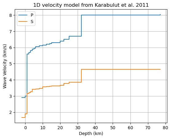
[5]:
ax = velocity_layers.plot(
    drawstyle="steps-post",
    ylabel="Wave Velocity (km/s)",
    xlabel="Depth (km)",
    title="1D velocity model from Karabulut et al. 2011",
    grid=True,
)
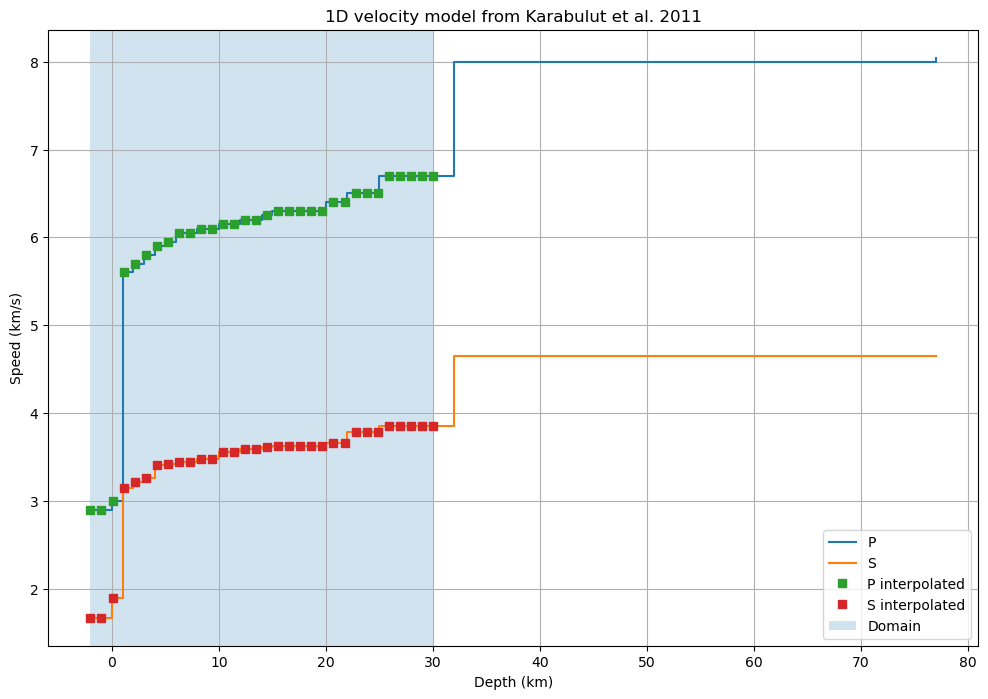
Interpolate velocity model at depth
We compute the travel times on a finer grid than the model grid, so we need to interpolate the model. We define 30 depths between 30 km and -2 km.
[6]:
depths = np.linspace(30.0, -2.0, 32)
Then we interpolate the velocity at the given depths using pandas.DataFrame method reindex.
[7]:
velocity_layers_interp = velocity_layers.reindex(depths, method="ffill")
We can then compare the natural (layered) and interpolated models as a function of depth
[8]:
velocity_layers.plot(drawstyle="steps-post")
velocity_layers_interp.sort_values("depth").plot(
    drawstyle="steps-post",
    xlabel="Depth (km)",
    ylabel="Speed (km/s)",
    title="1D velocity model from Karabulut et al. 2011",
    ax=plt.gca(),
    grid=True,
    figsize=(12, 8),
    marker="s",
    ls=""
)

# Labels and legends
plt.axvspan(depths.min(), depths.max(), alpha=0.2)
plt.legend(["P", "S", "P interpolated", "S interpolated", "Domain"])
plt.show()
Expand model laterally
Because pykonal uses three-dimensional coordinate systems, we need to cast the one-dimensional velocity model onto a three-dimensional grid. The following define the grid in the longitude and latitude dimensions.
[9]:
velocity_layers_interp
[9]:
| P | S | |
|---|---|---|
| depth | ||
| 30.000000 | 6.70 | 3.85 |
| 28.967742 | 6.70 | 3.85 |
| 27.935484 | 6.70 | 3.85 |
| 26.903226 | 6.70 | 3.85 |
| 25.870968 | 6.70 | 3.85 |
| 24.838710 | 6.50 | 3.78 |
| 23.806452 | 6.50 | 3.78 |
| 22.774194 | 6.50 | 3.78 |
| 21.741935 | 6.40 | 3.66 |
| 20.709677 | 6.40 | 3.66 |
| 19.677419 | 6.30 | 3.63 |
| 18.645161 | 6.30 | 3.63 |
| 17.612903 | 6.30 | 3.63 |
| 16.580645 | 6.30 | 3.63 |
| 15.548387 | 6.30 | 3.63 |
| 14.516129 | 6.25 | 3.61 |
| 13.483871 | 6.20 | 3.59 |
| 12.451613 | 6.20 | 3.59 |
| 11.419355 | 6.15 | 3.56 |
| 10.387097 | 6.15 | 3.56 |
| 9.354839 | 6.10 | 3.48 |
| 8.322581 | 6.10 | 3.48 |
| 7.290323 | 6.05 | 3.44 |
| 6.258065 | 6.05 | 3.44 |
| 5.225806 | 5.95 | 3.42 |
| 4.193548 | 5.90 | 3.41 |
| 3.161290 | 5.80 | 3.26 |
| 2.129032 | 5.70 | 3.21 |
| 1.096774 | 5.60 | 3.15 |
| 0.064516 | 3.00 | 1.90 |
| -0.967742 | 2.90 | 1.67 |
| -2.000000 | 2.90 | 1.67 |
[10]:
longitudes = np.linspace(30.20, 30.45, 25)
# sample latitudes in decreasing order to get corresponding colatitudes in increasing order (see explanation further)
latitudes = np.linspace(40.76, 40.60, 16)
We then expand the velocity vector in the longitude and latitude dimensions with xarray. This operation is automatically done with the expand_dim() method.
[11]:
velocity_P = np.zeros((len(depths), len(latitudes), len(longitudes)), dtype=np.float32)
velocity_S = np.zeros((len(depths), len(latitudes), len(longitudes)), dtype=np.float32)
# use numpy's broadcasting rules
velocity_P[...] = velocity_layers_interp["P"].values[:, None, None]
velocity_S[...] = velocity_layers_interp["S"].values[:, None, None]
# store the P- and S-wave velocity models in a dictionary
velocity_model = {
    "P": velocity_P,
    "S": velocity_S
}
Station coordinates
We extract the station coordinates from the XML files.
[12]:
# Get inventories
inventory = read_inventory("../data/processed/*xml")

# Extract stations
stations = [sta for net in inventory for sta in net]
attrs = "longitude", "latitude", "elevation", "code"
stations = [{item: getattr(sta, item) for item in attrs} for sta in stations]

# Turn into dataframe
network = pd.DataFrame(stations).set_index("code")
network["depth"] = -1e-3 * network.elevation

# Save network metadata
network.to_csv("../data/network.csv")

# Show
network
[12]:
| longitude | latitude | elevation | depth | |
|---|---|---|---|---|
| code | ||||
| DC06 | 30.265751 | 40.616718 | 555.0 | -0.555 |
| DC07 | 30.242170 | 40.667080 | 164.0 | -0.164 |
| DC08 | 30.250130 | 40.744438 | 162.0 | -0.162 |
| DD06 | 30.317770 | 40.623539 | 182.0 | -0.182 |
| DE07 | 30.411539 | 40.679661 | 40.0 | -0.040 |
| DE08 | 30.406469 | 40.748562 | 31.0 | -0.031 |
| SAUV | 30.327200 | 40.740200 | 170.0 | -0.170 |
| SPNC | 30.308300 | 40.686001 | 190.0 | -0.190 |
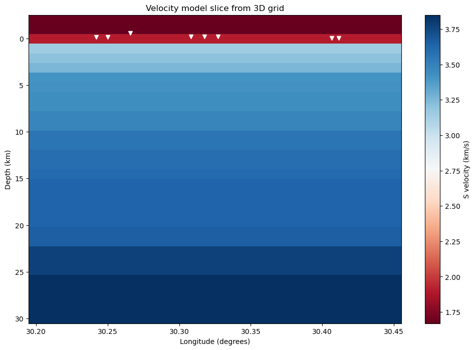
Show model and stations
This cell selects a slice of the velocity model with the DataArray.sel() and plots it.
[14]:
# Select slice at first latitude index
phase = "S"
velocities_slice = velocity_model[phase][:, 0, :]

# Show velocities
fig = plt.figure(figsize=(12, 8))
img = plt.pcolormesh(longitudes, depths, velocities_slice, cmap="RdBu")
cb = plt.colorbar(img)

# Show stations
plt.plot(network.longitude, network.depth, "wv")

# Labels
ax = plt.gca()
ax.set_xlabel("Longitude (degrees)")
ax.set_ylabel("Depth (km)")
ax.set_title("Velocity model slice from 3D grid")
cb.set_label(f"{phase} velocity (km/s)")
ax.invert_yaxis()
Compute travel times
The travel times are computed for every station with the Eikonal solver of pykonal. The travel times are then saved into a h5 file for later use.
Warning: For pykonal, we need to give the velocity grid in spherical coordinates \((r, \theta, \varphi)\), which is why we built the grid with decreasing depths and latitudes.
Spherical coordinates:
\(r\): Distance from center or Earth in km (= decreasing depth).
\(\theta\): Polar angle in radians (= co-latitude or, equivalently, decreasing latitude).
\(\varphi\): Azimuthal angle in radians (= longitude).
[15]:
STATION_ENTRIES = ["latitude", "longitude", "depth"]

# Initialize travel times
travel_times = {}

# Reference point
reference_point = geo2sph((latitudes.max(), longitudes.min(), depths.max()))
node_intervals = (
    np.abs(depths[1] - depths[0]),
    np.deg2rad(np.abs(latitudes[1] - latitudes[0])),
    np.deg2rad(longitudes[1] - longitudes[0]),
)

# Loop over stations and phases
for phase in velocity_model:
    travel_times[phase] = {}
    for station in tqdm.tqdm(network.index, desc=f"Travel times {phase}"):

        # Initialize Eikonal solver
        solver = PointSourceSolver(coord_sys="spherical")
        solver.velocity.min_coords = reference_point
        solver.velocity.node_intervals = node_intervals
        velocity = velocity_model[phase]
        solver.velocity.npts = velocity.shape
        solver.velocity.values = velocity.copy()

        # Source
        src_loc = network.loc[station][STATION_ENTRIES].values
        solver.src_loc = np.array(geo2sph(src_loc).squeeze())

        # Solve Eikonal equation
        solver.solve()

        # Update the travel_times dictionary
        tt = solver.tt.values
        # pykonal might produce a singularity at origin
        tt[np.isinf(tt)] = 0
        travel_times[phase][station] = tt
Travel times P:   0%|          | 0/8 [00:00<?, ?it/s]Travel times P: 100%|██████████| 8/8 [00:03<00:00,  2.01it/s]
Travel times S: 100%|██████████| 8/8 [00:03<00:00,  2.08it/s]
Save travel times and grid coordinates
Save the travel times as a hdf5 file. This format preserves a self-explanatory data structure and supports compression.
[16]:
# build 3D gridded coordinates from depths, latitudes and longitudes vectors
# these are the coordinates of the points in the travel time grid
depths_g, latitudes_g, longitudes_g = np.meshgrid(
    depths, latitudes, longitudes, indexing="ij"
)
[17]:
with h5.File("../data/travel_times.h5", mode="w") as ftt:
    ftt.create_group("source_coordinates")
    ftt["source_coordinates"].create_dataset("depth", data=depths_g)
    ftt["source_coordinates"].create_dataset("latitude", data=latitudes_g)
    ftt["source_coordinates"].create_dataset("longitude", data=longitudes_g)
    for phase in ["P", "S"]:
        ftt.create_group(phase)
        for sta in travel_times[phase]:
            ftt[phase].create_dataset(sta, data=travel_times[phase][sta])
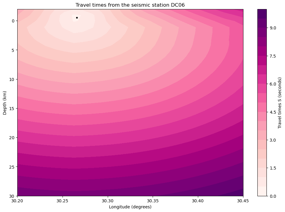
Show travel times at a given station
[18]:
CONTOUR_LEVELS = 20
SEISMIC_PHASE = "S"
station = network.loc["DC06"]

# Show
latitude_id = np.abs(latitudes - station.latitude).argmin()
time_delays = travel_times[SEISMIC_PHASE][station.name]
time_delays = time_delays[:, latitude_id, :]
fig = plt.figure(figsize=(12, 8))
img = plt.contourf(longitudes, depths, time_delays, cmap="RdPu", levels=CONTOUR_LEVELS)

# Colorbar
cb = plt.colorbar(img)
cb.set_label(f"Travel times {SEISMIC_PHASE} (seconds)")

# Station
plt.plot(station.longitude, station.depth, "k.")

# Labels
ax = plt.gca()
ax.invert_yaxis()
ax.set_xlabel("Longitude (degrees)")
ax.set_ylabel("Depth (km)")
ax.set_title(f"Travel times from the seismic station {station.name}")
plt.show()